Lab 12: Processing UAS Data in Pix4D

Introduction

The purpose of this lab was to provide an introduction to the Pix4D software package.  This involved constructing a point cloud data set, a true orthomosaic, and a digital surface model (DSM).  Additionally, the software was used to calculate surface area, volume and to create a video animation.  

Pix4D Overview
Pix4D software was founded in 2011 and is "committed to creating professional, georeferenced maps and models from drone imagery" (Pix4D website).  Pix4D is currently the premier software for constructing point clouds.  The software is very user-friendly and is used in many industries such as surveying, construction, agriculture and real estate.  To get a quick overview of how to use Pix4D software, check out the video below:

Video 1: YouTube video detailing how to use Pix4D

Study Area

The study area for this project was Litchfield Mine.  Using a Phantom drone, imagery was collected over the mining area by the course instructor.  Only a portion of the total area surveyed was processed in this activity (see Figure 1).  

Figure 1: Study area shown in Pix4D; area inside red box used for processing

Methods

Processing in Pix4D
After learning a bit about Pix4D from the instructor and browsing through the software manual, it was time to gain hands-on experience.  First, a new project was created within the software.  68 drone images of Litchfield Mine were then imported into Pix4D.  

To cut down on processing time, a small subset of the total imagery was selected for processing (as shown previously in Figure 1).   In Pix4D, there are three choices under Processing Options: Initial Processing, Point Cloud & Mesh, and DSM, Orthomosaic, and Index.  First, only Initial Processing was carried out to ensure that everything was running smoothly.  After this processing was finished, a Quality Report is generated in Pix4D.  This report provides the user with information about the camera and images at hand (see Figure 2, Figure 3).  Figure 3 illustrates the high level of image overlap present, which bodes well for future processing.  Areas of low overlap are located on the edges of the study area, which will not be a huge problem for processing. 

Figure 2: Quality Report summary in Pix4D

Figure 3: Quality Report map of image overlap

Then, after the Quality Report was determined to be satisfactory, the other two processing options (Point Cloud & Mesh and DSM, Orthomosaic, and Index) were run.  These two processing functions took about 10 minutes to run.  Had the selected study area been larger, the processing would have taken much longer.  

After processing was complete, the results were used to do the following: 

• Calculate the area of a surface within the Ray Cloud editor (Figure 4)
• Measure the length of a linear feature in the Ray Cloud editor
• Calculate the volume of a 3D object (Figure 5) 
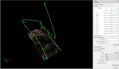
• Create an animation that flies over the study area (Figure 6, Video 2) 

Figure 4: Screenshot displaying a surface area calculation in Pix4D

Figure 5: Screenshot showing a volumetrics calculation of a sand pile in Pix4D

Figure 6: Screenshot depicting an animation flight path in Pix4D

Video 2: Animation created in Pix4D showing "fly over" of study area

Processing in ArcGIS
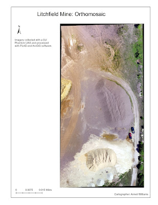
Upon completion of processing in Pix4D, the resulting DSM and orthomosaic were visualized in ArcGIS (Figure 7, Figure 8).  A hillshade was used in conjunction with the DSM to make the elevation differences more discernible.  

Figure 7: Map showing DSM of Litchfield Mine imagery

Figure 8: Map showing orthomosaic of Litchfield Mine imagery

Conclusion & Review of Pix4D

This exercise provided a great introduction to using Pix4D.  Judging from this basic activity, Pix4D appears to be an effective and easy-to-use software.  One major downfall of the software is the processing time, which could be extremely long for larger study areas.  Since many industries outside of the geospatial arena are using the software (for example, real estate), the user-friendly nature of the software is crucial.  Pix4D also provides lots of excellent online resources such as their Software Manual and Help to help less experienced users.  More experience with the software would be necessary to give a complete review.  

Lab 11: GPS Topographic Survey

Introduction

The purpose of this lab was to gain experience in collecting data with a high precision GPS unit.  The study area was a grassy knoll located on the UW-Eau Claire campus. 

Methods

In this lab, data was collected using a Topcon HiPer high precision GPS unit with a Tesla field controller (see Figure 1).  Due to complications with the geography department's ArcGIS account, the class was only able to collect 20 elevation points total.  Points were collected by two students at a time in a random survey throughout the grassy knoll.  Each student took a turn operating the Topcon HiPer and the field controller.  After all of the data was collected, the instructor was imported as a text file for future use in ArcGIS. 

To better visualize the elevation of the knoll, a number of interpolation methods were used, namely TIN, Natural Neighbor, Spline, IDW, and Kriging interpolation. 

Figure 1: Picture showing class members operating the Topcon HiPer

Results & Discussion

The results of the interpolations all were different, with various advantages and disadvantages.  To read more about the pros and cons of each interpolation method, check out Lab 5: Visualizing Terrain Survey.  The spline interpolation appears to provide the best visualization of the actual terrain. 

One of the main sources of error in the interpolation maps was the fact that the data was entered in as if it was in UTM Zone 16, when it should have been Zone 15.  This caused some distortion.  After importing the data as a text file, some of the fields were also mislabeled, which caused some confusion.  Despite this, all of the interpolations were performed successfully. 

Figure 2: TIN interpolation

Figure 3: IDW interpolation

Figure 4: Kriging interpolation

Figure 5: Natural Neighbor interpolation

Figure 6: Spline interpolation

Conclusion

This lab provided a good introduction to using a high precision GPS unit.  Ideally, each student would have been able to collect more than just two points to gain more experience, but the class made do.  Additionally, the UTM zone fiasco proved that it is important to be very careful when setting everything up for data entry on the field controller.